Changing the Endpoint Address of an RHQ Storage Node

There is very limited support for changing the endpoint address of a storage node. In fact the only way to do so is by undeploying and redeploying the node with the new address. And in some cases, like when there is only a single storage node, this is not even an option. BZ 1103841 was opened to address this, and the changes will go into RHQ 4.13.

Changing the endpoint address of a Cassandra node is a routine maintenance operation. I am referring specifically to the address on which Cassandra uses for gossip. This address is specified by the listen_address property in cassandra.yaml. The key thing when changing the address is to ensure that the node's token assignments do not change. Rob Coli's post on changing a node's address provides a nice summary of the configuration changes involved.

With CASSANDRA-7356 however, things are even easier. Change the value of listen_address and restart Cassandra with the following system properties defined in cassandra-env.sh,

• -Dcassandra.replace_address=<new_address>
• -Dcassandra.replace_address_first_boot=true 

The seeds property in cassandra.yaml might need to be updated as well. Note that there is no need to worry about the auto_bootstrap, initial_token, or num_tokens properties.

For the RHQ Storage Node, these system properties will be set in cassandra-jvm.properties. Users will be able to update a node's address either through the storage node admin UI or through the RHQ CLI. One interesting to note is that the RHQ Storage Node resource type uses the node's endpoint address as its resource key. This is not good. When the address changes, the agent will think it has discovered a new Storage Node resource. To prevent this we can add resource upgrade support in the rhq-storage plugin, and change the resource key to use the node's host ID which is a UUID that does not change. The host ID is exposed through the StorageServiceMBean.getLocalHostId JMX attribute.

If you interested in learning more about the work involved with adding support for changing a storage node's endpoint address, check out the wiki design doc that I will be updating over the next several days.

Upgrading to RHQ 4.9

RHQ 4.8 introduced the new Cassandra backend for metrics. There has been a tremendous amount of work since then focused on the management of the new RHQ Storage Node. We do want to impose on users the burden of managing a second database. One of our key goals is to provide robust management such that Cassandra is nothing more than an implementation detail for users.

The version of Cassandra shipped in RHQ 4.8 includes some native libraries. One of the main uses for those native libraries is compression.  If the platform on which Cassandra is running has support for the native libraries, table compression will be enabled. Data files written to disk will be compressed.

All of the native libraries have been removed from the version of Cassandra shipped in RHQ 4.9. The reason for this change is to ensure RHQ continues to provide solid cross-platform support. The development and testing teams simply do not have the bandwidth right now to maintain native libraries for all of the supported platforms in RHQ and JON.

The following information applies only to RHQ 4.8 installs.

Since RHQ 4.9 does not ship with native those compression libraries, Cassandra will not be able to decompress the data files on disk.

Compression has to be disabled in your RHQ 4.8 installation before upgrading to 4.9. There is a patch which you will need to run prior to upgrading. Download rhq48-storage-patch.zip and follow the instructions provided in rhq48-storage-patch.sh|bat.

I do want to mention that we will likely re-enable compression using a pure Java compression library in a future RHQ release.

Configuring Cassandra JDBC with JBoss AS 7

1. Build the driver source

cassandra-jdbc is not yet available in the public Maven repos so it has to be built from source. There is already an open ticket requesting that the artifacts get published to a public Maven repo. If you do not already have a copy of the source, clone the git repo,

git clone https://code.google.com/a/apache-extras.org/p/cassandra-jdbc/

Build the project,

mvn install -DskipTests

cassandra-jdbc uses Maven. This generate artifacts and installs them into the local Maven repository. I set the skipTests property to tell Maven not to execute any tests. There are some failures in my local repo I have yet to investigate.

2. Determine runtime dependencies

We need to determine the runtime dependencies for the driver so that we know what libraries need to be installed in the next step. The Maven dependency plugin makes this easy. Run the following,

mvn dependency:copy-dependencies -DincludeScope="runtime"

This generates a list of the runtime dependencies under <CASSANDRA_JDBC_HOME>/target/dependency. You should find the following:

• cassandra-clientutil-1.2.0-beta1.jar
• cassandra-thrift-1.2.0-beta1.jar
• commons-lang-2.4.jar
• guava-12.0.jar
• jsr305-1.3.9.jar
• libthrift-0.7.0.jar
• slf4j-api-1.6.1.jar

3. Create the JBoss module

There are several ways to install to the driver in JBoss AS 7. I am going to describe creating a module since that is what I have done. As it turns out JBoss AS 7 already comes with modules for some of the dependencies; so, we will not include all dependencies in the above list in the module we create. First we need to create the module directory tree.

mkdir -p <JBOSS_HOME>/modules/org/apache-extras/cassandra-jdbc/main

Then copy the cassandra-jdbc build artifact.

cp <CASSANDRA_JDBC_HOME>/target/cassandra-jdbc-1.2.0-SNAPSHOT.jar <JBOSS_HOME>/modules/org/apache-extras/cassandra-jdbc/main 

Now copy the following dependencies to the module directory, right along side the driver JAR file.

• cassandra-clientutil-1.2.0-beta1.jar
• cassandra-thrift-1.2.0-beta1.jar
• guava-12.0.jar
• jsr305-1.3.9.jar

Do not copy slf4j-api or commons-lang because they are already installed as modules. There is also a module for guava as well, but it is an earlier version; consequently, we include guava in our module so that we have the correct version. Now create a module.xml to define the module resources and dependencies. This file goes in the same directory as the JAR file dependencies and it should look like,

That's it for creating the module. All that is left to do is define the data source and driver.

4. Declare and configure driver and data source

Open <JBOSS_HOME>/standalone/configuration/standalone.xml and scroll down until you reach the data sources subsystem which starts with the tag <subsystem xmlns="urn:jboss:domain:datasources:1.0"> We need to declare a data source as well as a driver. Here is what my additions look like,

This is a minimal configuration for illustration purposes. Changes were recently pushed to the cassandra-jdbc repo to provide more support for connection pooling. For the data source class we could also use org.apache.cassandra.cql.jdbc.PooledCassandraDataSource. Notice in the connection URL that the is a version parameter to tell the server we are using CQL v3. Take a look at the user guide for a full listing of available configuration options for data sources and drivers.

5. Start JBoss AS and verify data source configuration

In a terminal go to <JBOSS_HOME>/bin and then run ./standalone.sh. Now log into the web console at http://localhost:9990. Click on the Profile link in the upper right corner. Then click on Datasources in the menu on the left and you should see something like this,

Finally select the Connection tab and click the Test Connection button as shown below.

We are all set now to use the data source in application code. We can use resource injection just as we would with any other data source.

Why I am ready to move to CQL for Cassandra application development

Earlier this year, I started learning about Cassandra as it seemed like it might be a good fit as a replacement data store for metrics and other time series data in RHQ. I developed a prototype for RHQ. I used the client library Hector for accessing Cassandra from within RHQ. I defined my schema using a Cassandra CLI script. I recall when I first read about CQL. I spent some time deliberating over whether to define the schema using a CLI script or using a CQL script. Although I was intrigued but ultimately decided against using CQL. As the CLI and the Thrift interface were more mature, it seemed like the safer bet. While I decided not to invest any time in CQL, I did make a mental note to revisit it at a later point since there was clearly a big emphasis within the Cassandra community for improving CQL. That later point is now, and I have decided to start making extensive use of CQL.

After a thorough comparative analysis, the RHQ team decided to move forward with using Cassandra for metric data storage. We are making heavy use of dynamic column families and wide rows. Consider for example the raw_metrics column family in figure 1,

Figure 1. raw_metrics column family

The metrics schedule id is the row key. Each data point is stored in a separate column where the metric timestamp is the column name and the metric value is the column value. This design supports fast writes as well as fast reads and works particularly well for the various date range queries in RHQ. This is considered a dynamic column family because the number of columns per row will vary and because column names are not defined up front. I was quick to rule out using CQL due to a couple misconceptions about CQL's support for dynamic column families and wide rows. First, I did not think it was possible to define a dynamic table with wide rows using CQL. Secondly, I did not think it was possible to execute range queries on wide rows.

A couple weeks ago I came across this thread on the cassandra-users mailing list which points out that you can in fact create dynamic tables/column families with wide rows. And conveniently after coming across this thread, I happened to stumble on the same information in the docs. Specifically the DataStax docs state that wide rows are supported using composite column names. The primary key can have multiple components, but there must be at least one column that is not part of the primary key. Using CQL I would then define the raw_metrics column family as follows,

This CREATE TABLE statement is straightforward, and it does allow for wide rows with dynamic columns. The underlying column family representation of the data is slightly different from the one in figure 1 though.

Figure 2. CQL version of raw_metrics column family

Each column name is now a composite that consists of the metric timestamp along with the string literal, value. There is additional overhead on reads and writes as the column comparator now has to compare the string in addition to the timestamp. Although I have yet to do any of my own benchmarking, I am not overly concerned by the additional string comparison. I was however concerned about the additional overhead in terms of disk space. I have done some preliminary analysis and concluded that the difference with just storing the timestamp in the column name is negligible due to compression of SSTables which is enabled by default.

My second misconception about executing range queries is really predicated on the first misconception. It is true that you can only query named columns in CQL; consequently, it is not possible to perform a date range query against the column family in figure 1. It is possible though to execute a date range query against the column family in figure 2.

RHQ supports multiple upgrade paths. This means that in order to upgrade to the latest release (which happens to be 4.5.0 at the time of this writing), I do not have to first upgrade to the previous release (which would be 4.4.0). I can upgrade from 4.2.0 for instance. Supporting multiple upgrade paths requires a tool for managing schema changes. There are plenty of such tools for relational databases, but I am not aware of any for Cassandra. But because we can leverage CQL and because there is a JDBC driver, we can look at using an existing tool instead of writing something from scratch. I have done just that and working on adding support for Cassandra to Liquibase. I will have more on that in future post. Using CQL allows us to reuse existing solutions which in turn is going to save a lot of development and testing effort.

The most compelling reason to use CQL is the familiar, easy to use syntax. I have been nothing short of pleased with Hector. It is well designed, the online documentation is solid, and the community is great. Whenever I post a question on the mailing list, I get responses very quickly. With all that said, contrast the following two, equivalent queries against the raw_metrics column family.

RHQ developers can look at the CQL version and immediately understand it. Using CQL will result in less, easier to maintain code. We can also leverage ad hoc queries with cqlsh during development and testing. The JDBC driver also lends itself nicely to applications that run in an application as RHQ does.

Things are still evolving both with CQL and with the JDBC driver. Collections support is coming in Cassandra 1.2. The JDBC driver does not yet support batch statements. This is due to the lack of support for it the server side. The functionality is there in the Cassandra trunk/master branch, and I expect to see it in the 1.2 release. The driver also currently lacks support for connection pooling. These and other critical features will surely make their way into the driver. With the enhancements and improvements to CQL and to the JDBC driver, adding Cassandra support to Hibernate OGM becomes that much more feasible.

The flexibility, tooling, and ease of use make CQL a very attractive option for working with Cassandra. I doubt the Thrift API is going away any time soon, and we will continue to leverage the Thrift API through Hector in RHQ in various places. But I am ready to make CQL a first class citizen in RHQ and look forward to watching it continue to mature into a great technology.

Setting up a local Cassandra cluster using RHQ

As part of my ongoing research into using Cassandra with RHQ, I did some work to automate setting up a Cassandra cluster (for RHQ) on a single machine for development and testing. I put together a short demo showing what is involved. Check it out at http://bit.ly/N3jbT8.

Aggregating Metric Data with Cassandra

Introduction

I successfully performed metric data aggregation in RHQ using a Cassandra back end for the first time recently. Data roll up or aggregation is done by the data purge job which is a Quartz job that runs hourly. This job is also responsible for purging old metric data as well as data from others parts of the system. The data purge job invokes a number of different stateless session EJBs (SLSBs) that do all the heavy lifting. While there is a still a lot of work that lies ahead, this is a big first step forward that is ripe for discussion.

Integration

JPA and EJB are the predominant technologies used to implement and manage persistence and business logic. Those technologies however, are not really applicable to Cassandra. JPA is for relational databases and one of the central features of EJB is declarative, container-managed transactions. Cassandra is neither a relational nor a transactional data store. For the prototype, I am using server plugins to integrate Cassandra with RHQ.

Server plugins are used in a number of areas in RHQ already. Pluggable alert notifcation senders is one of the best examples. A key feature of server plugins is the encapsulation made possible by the class loader isolation that is also present with agent plugins. So let's say that Hector, the Cassandra client library, requires a different version of a library that is already used by RHQ. I can safely use the version required by Hector in my plugin without compromising the RHQ server. In addition to the encapsulation, I can dynamically reload my plugin without having to restart the whole server. This can help speed up iterative development.

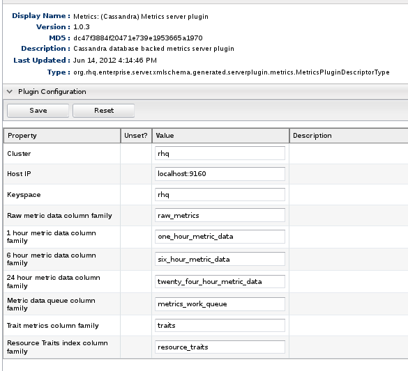
Cassandra Server Plugin Configuration

You can define a configuration in the plugin descriptor of a server plugin. The above screenshot shows the configuration of the Cassandra plugin. The nice thing about this is that it provides a consistent, familiar interface in the form of the configuration editor that is used extensively throughout RHQ. There is one more screenshot that I want to share.

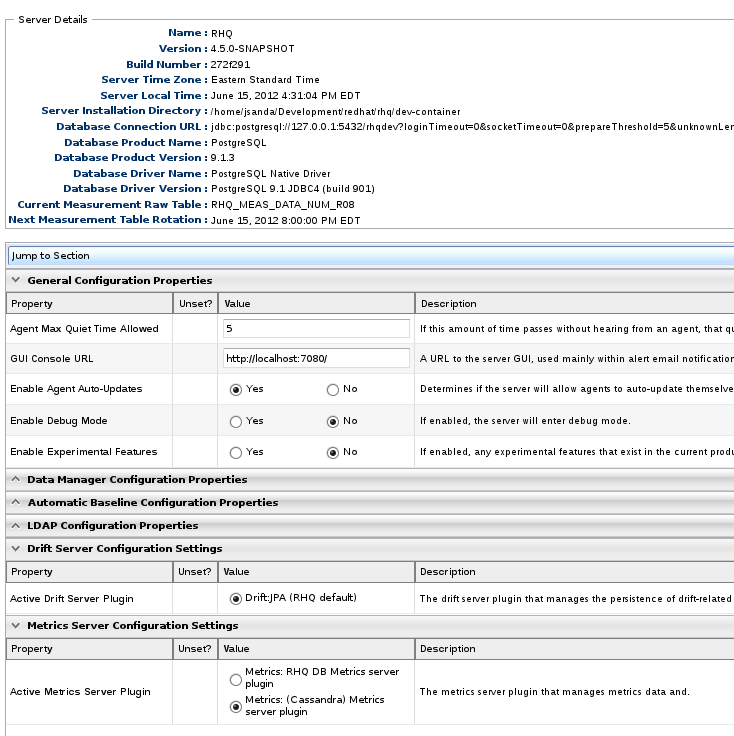
System Settings

This is a screenshot of the system settings view. It provides details about the RHQ server itself like the database used, the RHQ version, and build number. There are several configurable settings, like the retention period for alerts and drift files and settings for integrating with an LDAP server for authentication. At the bottom there is a property named Active Metrics Server Plugin. There are currently two values from which to choose. The first is the default, which uses the existing RHQ database. The second is for the new Cassandra back end. The server plugin approach affords us a pluggable persistence solution that can be really useful for prototyping among other things. Pluggable persistence with server plugins is a really interesting topic in and of itself. I will have more to say on that in future post.

Implementation

The Cassandra implementation thus far uses the same buckets and time slices as the existing implementation. The buckets and retention periods are as follows:

Metrics Data Bucket	Data Retention Period
raw data	7 days
one hour data	2 weeks
6 hour data	1 month
1 day data	1 year

Unlike the existing implementation, purging old data is accomplished simply by setting the TTL (time to live) on each column. Cassandra takes care of purging expired columns. The schema is pretty straightforward. Here is the column family definition for raw data specified as a CLI script:


The row key is the metric schedule id. The column names are timestamps and column values are doubles. And here is the column family definition for one hour data:


As with the raw data, the schedule id is the row key. Unlike the raw data however, we use composite columns here. All the buckets with the exception of the raw data, store computed aggregates. RHQ calculates and stores the min, max, and average for each (numeric) metric schedule. The column name consists of a timestamp and an integer. The integer identifies whether the value is the max, min, or average. Here is some sample (Cassandra) CLI output for one hour data:


Each row in the output reads like a tuple. The first entry is the column name with a colon delimiter. The timestamp is listed first followed by the integer code to identify the aggregate type. Next is the column value, which is the value of the aggregate calculation. Then we have a timestamp. Every column has a timestamp in Cassandra has a timestamp. It is used for conflict resolution on writes. Lastly, we have the ttl. The schema for the remaining buckets is similar the one_hour_metric_data column family so I will not list them here.

The last implementation detail I want to discuss is querying. When the data purge job runs, it has to determine what data is ready to be aggregated. With the existing implementation that uses the RHQ database, queries are fast and efficient using indexes. The following column family definition serves as an index to make queries fast for the Cassandra implementation as well:


The row key is the metric data column family name, e.g., one_hour_metric_data. The column name is a composite that consists of a timestamp and a schedule id. Currently the column value is an integer that is always set to zero because only the column name is needed. At some point I will likely refactor the data type of the column  value to something that occupies less space. Here is a brief explanation of how the index is used. Let's start with writes. Whenever data for a schedule is written into one bucket, we update the index for the next bucket. For example, suppose data for schedule id 123 is written into the raw_metrics column family at 09:15. We will write into the "one_hour_metric_data" row of the index with a column name of 09:00:123. The timestamp in which the write occurred is rounded down to the start of the time slice of the next bucket. Further suppose that additional data for schedule 123 is written into the raw_metrics column family at times 09:20, 09:25, and 09:30. Because each of those timestamps gets rounded down to 09:00 when writing to the index, we do not wind up with any additional columns for that schedule id. This means that the index will contain at most one column per schedule for a given time slice in each row.

Reads occur to determine what data if any needs to be aggregated. Each row is in the index is queried. After a column is read and the data for the corresponding schedule is aggregated into the next bucket, that column is then deleted. This index is a lot like a job queue. Reads in the existing implementation that use a relational database should be fast; however, there is still work that has to be done to determine what data if any needs to be aggregated when the data purge job runs. With the Cassandra implementation, the presence of a column in a row of the metrics_aggregates_index column family indicates that data for the corresponding schedule needs to be aggregated.

Testing

I have pretty good unit test coverage, but I have only done some preliminary integration testing. So far it has been limited to manual testing. This includes inspecting values in the database via the CLI or with CQL and setting break points to inspect values. As I look to automate the integration testing, I have been giving some thought to how metric data is pushed to the server. Relying on the agent to push data to the server is sub optimal for a couple reasons. First, the agent sends measurement reports to the server once a minute. I need better control of how frequently and when data is pushed to the server.

The other issue with using the agent is that it gets difficult to simulate older metric data that has been reported over a specified duration, be it an hour, a day, or a week. Simulating older data is needed for testing that data is aggregated into 6 hour and 24 hour buckets and that data is purged at appropriate times.

RHQ's REST interface is a better fit for the integration testing I want to do. It already provides the ability to push metric data to the server. I may wind up extending the API, even if just for testing, to allow for kicking off the aggregation that runs during the data purge job. I can then use the REST API to query the server and verify that it returns the expected values.

Next Steps

There is still plenty of work ahead.I have to investigate what consistency levels are most appropriate for different operations. There is a still a large portion of the metrics APIs that needs to be implemented, some of the more important ones being query operations used to render metrics graphs and tables. The data purge job is not the best approach going forward for doing the aggregation. Only a single instance of the job runs each hour, and it does not exploit any of the opportunities that exist for parallelism. Lastly and maybe most importantly, I have yet to start thinking about how to effectively manage the Cassandra cluster with RHQ. As I delve into these other areas I will continue sharing my thoughts and experiences.

Modeling Metric Data in Cassandra

RHQ supports three types of metric data - numeric, traits, and call time. Numeric metrics include things like the amount of free memory on a system or the number of transactions per minute. Traits are strings that track information about a resource and typically change in value much less frequently than numeric metrics. Some examples of traits include server start time and server version. Call time metrics capture the execution time of requests against a resource. An example of call time metrics is EJB method execution time.

I have read several times that with Cassandra it is best to let your queries dictate your schema design. I recently  spent some time thinking about RHQ's data model for metrics and how it might look in Cassandra. I decided to focus only on traits for the time being, but much of what I discuss applies to the other metrics types as well.

I will provide a little background on the existing data model to make it easier to understand some of the things I touch on. All metric data in RHQ belongs to resources. A particular resource might support metrics like those in the examples above, or it might support something entirely different. A resource has a type, and the resource type defines which type of metrics that it supports.We refer to these as measurement definitions. These measurement definitions, along with other meta data associated with the resource type, are defined in the plugin descriptor of the plugin that is responsible for managing the resource. You can think of a resource type of an abstraction and a resource is a realization of that abstraction. Similarly, a measurement definition is an abstraction, and a measurement schedule is a realization of a measurement definition. A resource can have multiple measurement schedules, and each schedule is associated with measurement definition. The schedule has a number of attributes like the collection interval, an enabled flag, and the value. When the agent reports metric data to the RHQ server the data is associated with a particular schedule. To tie it all together, here is a snippet of some of the relevant parts of the measurement classes:

To review, for a given measurement schedule, we can potentially add an increasing number of rows in the RHQ_MEASUREMENT_DATA_TRAIT table over time. There are a lot of fields included in the snippet for MeasurementDefinition. I chose to include most of them because they are pertinent to the discussion.

For the Cassandra integration, I am interested primarily in the MeasurementDataTrait class. All of the other types are managed by the RHQ database. Initially when I started thinking about what column families I would need, I felt overcome with writer's block. Then I reminded myself to think about trait queries and try to let those guide my design. I decided to focus on some resource-level queries and leave others like group-level queries for a later exercise. Here is a screenshot of one of the resource-level views where the queries are used:

Let me talk a little about this view. There are a few things to point out in order to understand the approach I took with the Cassandra schema. First, this is a list view of all the resource's traits. Secondly, the view shows only the latest value for each trait. Finally, the fields required by this query span across multiple tables and include resource id, schedule id, definition id, display name, value, and time stamp. Because the fields span across multiple tables, one or more joins is required for this query. There are two things I want to accomplish with the column family design in Cassandra. I want to be able to fetch all of the data with a single read, and I want to be able to fetch all of the traits for a resource in that read. Cassandra of course does not support joins; so, some denormalization is needed to meet my requirements. I have two column families for storing trait data. Here is the first one that supports the above list view as a Cassandra CLI script:

create column family resource_traits
    with comparator = 'CompositeType(DateType, Int32Type, Int32Type, BooleanType, UTF8Type, UTF8Type)' and
    default_validation_class = UTF8Type and
    key_validation_class = Int32Type;

The row key is the resource id. The column names are a composite type that consist of the time stamp, schedule id, definition id, enabled flag, display type, and display name. The column value is a string and is the latest known value of the trait. This design allows for the latest values of all traits to be fetched in a single read. It also gives me the flexibility to perform additional filtering. For example, I can query for all traits that are enabled or disabled. Or I can query for all traits whose values last changed after a certain date/time. Before I talk about the ramifications of the denormalization I want to introduce the other column family that tracks the historical data. Here is the CLI script for it:

create column family traits
    with comparator = DateType and
    default_validation_class = UTF8Type and
    key_validation_class = Int32Type;

This column family is pretty straightforward. The row key is the schedule id. The column name is the time stamp, and the column value is the trait value. In the relational design, we only store a new row in the trait table if the value has changed. I have only done some preliminary investigation, and I am not yet sure how to replicate that behavior with a single write. I may need to use a custom comparator. It is something I have to revisit.

I want to talk a little bit about the denormalization. As far this example goes, the system of record for everything except the trait data is the RHQ database. Suppose a schedule is disabled. That will now require a write to both the RHQ database as well as to Cassandra. When a new trait value is persisted, two writes have to be made to Cassandra - one to add a column to the traits column family and one to update the resource_traits column family.

The last thing I will mention about the design is that I could have opted for a more row based approach where each column in resource_traits is stored in a separate row. With that approach, I would use statically named columns like scheduleId and the corresponding value would be something like 1234. The primary reason I decided against this is because the RandomPartitioner is used for the partitioning strategy, which happens to be the default. RandomPartitioner is strongly recommended for most cases to allow for even key distribution across nodes. Without going into detail, range scans, i.e., row-based scans, are not possible when using the RandomPartitioner. Additionally, Cassandra is designed to perform better with slice queries, i.e., column-based queries than with range queries.

The design may change as I get further along in the implementation, but it is a good starting point. The denormalization allows for efficient querying of a resource's traits and offers the flexibility for additional filtering. There are some trade offs that have to be made, but at this point, I feel that they are worthwhile. One thing is for certain. Studying the existing (SQL/JPA) queries and understanding what data is involved and how helped flush out the column family design.